MagSat (Magnetic Field Satellite)

MagSat (Magnetic Field Satellite) /AEM-3 / Explorer 61

MagSat was a joint NASA and USGS (United States Geological Survey) mission, also known as AEM-3 (Applications Explorer Mission-3) and as Explorer 61. The overall objective was to obtain a first quantitative survey of the Earth's magnetic field (collection of data for improved modeling of the time-varying magnetic field generated within the core of the Earth, and to map variations in the strength and vector characteristics of crustal magnetization). ^{1) 2)}

Background

Prior to the spaceage, magnetic data from many geographic regions were simply nonexistent or sparse. The POGO (Polar Orbiting Geophysical Observatory) and the OGO (Orbiting Geophysical Observatories) 2, 4, and 6 satellites of NASA made global measurements of the scalar field from October 1965 through June 1971, and several geomagnetic field models based on POGO data were published. Their magnetometers provided measurements of the scalar field magnitude approximately every half second over an altitude range of ~ 400 to 1,500 km. ^{3) 4)}

Early in the POGO era, it was thought to be impossible to map crustal anomalies from space. However, while analyzing data from POGO, investigators discovered that the lower altitude data contained separable fields because of anomalies in Earth's crust, thus allowing for the development of a new class of investigations. Magsat data enhanced POGO data in two areas:

1) Vector measurements were used to determine the directional characteristics of anomaly regions and resolved ambiguities in their interpretation.

2) Lower altitude data provided increased signal strength and resolution for detailed studies of crustal anomalies.

Spacecraft

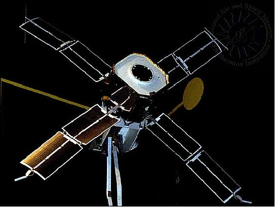
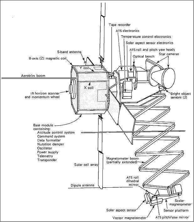
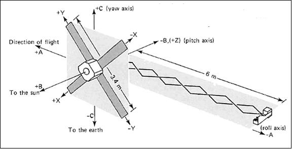
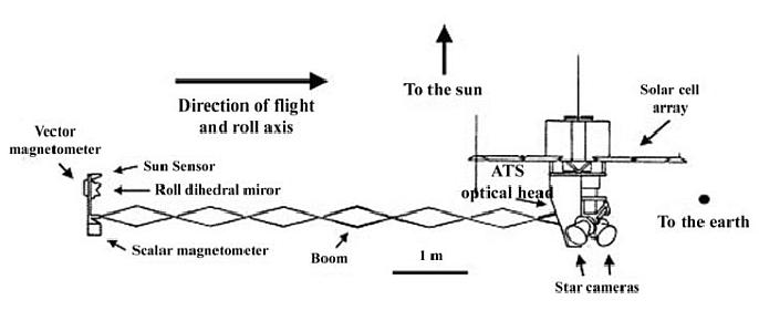
The spacecraft, designed, built and integrated by JHU/APL (Laurel, MD) for NASA, consists of two distinct parts: the payload module and the base module [containing the subsystems for data handling, power (4 solar panels), communications, commanding, and attitude control]. The instrument module houses a scalar and a vector magnetometer, two star cameras and the ATS (Attitude Transfer System) which is used to determine the relative orientation of the star cameras and the vector magnetometer. ⁵⁾

Magsat was intended to measure the vector components of the Earth's field to an accuracy of 0.01%; this meant that the orientation of the vector sensors must be known to 15 arcsec accuracy. The star cameras were good to an accuracy of 10 arcsec, but they had 2 kg of essential magnetic shielding that would distort the magnetic field . An extendable boom was needed to put the vector sensors 6 m away from the magnetic disturbance caused by the star cameras. But it was not possible for the boom to be mechanically stable to 5 arcsec. A system was needed to measure the orientation of the vector sensors relative to the star cameras. This system, the ATS, used an optical technique involving mirrors attached to the vector sensor to make the necessary measurement (Ref. 1).

The elements of the ATS and the two star cameras had to be tied together mechanically in some permanent and extremely stable fashion. The structure to achieve this was the optical bench, a built-up assembly of graphite fiber and epoxy resin that provided a near-zero coefficient of thermal expansion. The bench was attached to the satellite at five points, two of which were released by pyrotechnic devices after the satellite was in orbit. The three remaining support points did not apply stress to the bench. Heaters and temperature sensors at eight places stabilized the bench temperature at 25°C.

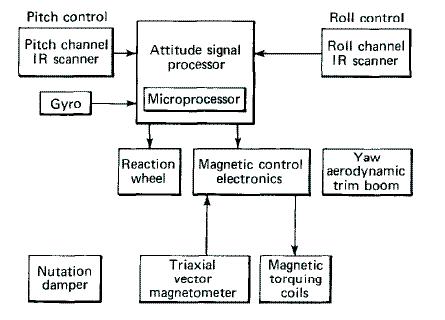
ACS (Attitude Control Subsystem): The spacecraft is 3-axis stabilized with the magnetometer boom trailing aft. The ACS maintains orientation to the local vertical coordinate system by using a momentum biased infrared scanner/reaction wheel and magnetic torquing for initial orientation and occasional control. A pitch axis rate gyro, sun sensors, coarse magnetometers, and the horizon scanner provide attitude and rate information for ground or on-board semiautonomous microprocessor control. MagSat used for the first time a set of microprocessors [RCA-1802 microprocessor, also known as COSMAC (Complementary Symmetry Monolithic Array Computer)] for the attitude and command subsystems. The RCA-1802 was radiation-hardened and applied low-power CMOS technology. Both the Intel 8080 and the RCA-1802 were 8-bit processors with clock rates of about 1 MHz. By the time these systems were launched, more powerful systems (e.g., Intel 8085 and 8086) had been commercially released but were not yet available in radiation-hardened form. - Note: The first spaceborne microprocessor (Intel 8080) was flown on the SEASAT mission of NASA/JPL (launch June 27, 1978). ^{6) 7) 8) 9) 10) 11)}

Spacecraft structure: The base module of MagSat is comprised of spare parts from the SAS-3 (Small Astronomy Satellite-3) spacecraft, built by JHU/APL in 1975. SAS-3 utilized a Doppler tracking system for position determination and had two star trackers that could provide attitude information to 10 arcseconds. - However, the magnetic fields associated with these star trackers and the spacecraft itself would have introduced unacceptable large errors into the magnetic field determinations. Therefore, a deployable scissors boom and an infrared ATS were developed for MagSat that put the scalar and vector magnetometers 6 m away from the star trackers and the body of the spacecraft.

MagSat spacecraft mass of 182 kg; spacecraft size = 1.55 m in height (3.4 m in deployed configuration, 4 solar panels). Planned mission life of 6 months (Ref. 11). ¹²⁾

Instrument module: height: 874 cm with trim boom extended, diameter: 77 cm with solar panels and magnetometer boom extended, width: 340 cm tip to tip with solar array deployed, length: 722 cm along flight path with magnetometer boom and solar array deployed. Base module: diameter: 66 cm, height: 61 cm.

EPS (Electrical Power Subsystem): An array of silicon solar cells mounted on four deployable panels generated electrical power for the MagSat spacecraft. The deployed panels formed a planar cruciform array, with the long axis of each panel perpendicular to the spacecraft B axis. The spacecraft battery consisted of 12 series-connected 8 Ahr NiCd (Nickel-Cadmium) cells operating at a nominal voltage of 16.7 V. The battery supplied energy to meet brief demands in excess of the generating capability of the solar array and operated the spacecraft during transient phases of orbit acquisition and attitude adjustment. It also sustained operation of the spacecraft during periods of solar eclipse that occurred late in the mission lifetime (Ref. 1).

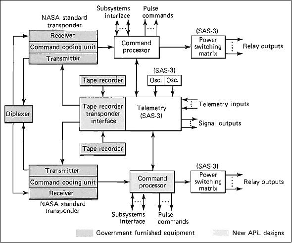
RF communications: The Magsat telecommunications system is based on the SAS-3 (Small Astronomy Satellite) with newly designed telemetry modulation control and recorder interface electronics. A microprocessor-based design for the Magsat command subsystem offers expanded capabilities and increased flexibility in real-time and delayed commanding operations. ¹³⁾

MagSat tape recorders: Tape recording the real-time telemetry data ensured that no information was lost during the time the spacecraft was out of contact with a ground receiving station. Two recorders, manufactured by Odetics Corp., recorded up to 9 x 10⁷ bit each, over a 12.5 hour maximum period. Upon command, the accumulation of data was played back to the ground at 312 kbit/s, which is 160 times the rate at which it was recorded. This took less than 4.7 minutes, well within the 6 to 10 minute duration of a satellite pass over a ground station.

Launch

A launch of MagSat took place on Oct. 30, 1979 on a Scout-G vehicle from VAFB, CA, USA.

Orbit: Sun-synchronous polar orbit; inclination=96.8º; perigee=350 km, apogee=551 km, period = 93.6 minutes.

Note: The selection of a sun-synchronous orbit of Magsat, resulting in a sampling of the magnetic field only at dawn and dusk local time, was a compromise dictated by the carrying capacity of the Scout launch vehicle. The chosen orbit, and mission lifetime (fall 1979 through spring 1980) allowed for a maximum exposure of the fixed solar array to the sun, a near-constant thermal environment, and a fixed flight attitude that allowed the star trackers to always face away from the Earth.

Mission Status

• MAGSAT collected scalar (total-field) and three orthogonal vector components of the magnetic field. The satellite remained in orbit for seven and a half months until June 11, 1980. The satellite provided the first precise measurements of the global magnetic field obtained so far, and the first measurements of the vector field in low-Earth orbit (LEO).

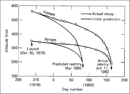
Legend to Figure 8: The decay was slower than predicted because the density of the atmosphere was less than expected. The satellite reentered on June 11, 1980.

• On April 12, 1980, eclipsing of Magsat by the Earth began, as predicted. The loss of solar array power during the eclipse meant that the satellite systems were entirely dependent on the stored energy in the nickel-cadmium battery. The battery voltage dropped much more rapidly than the project expected during the eclipse. After the data were analyzed it became apparent that the battery capacity had dropped to about 12% of its nominal capacity of 8 Ahr. This loss in capacity has been ascribed to the "memory" effect associated with shallow discharging of nickel-cadmium batteries (which occurred prior to the eclipsing period) and also to simultaneous exposure to elevated temperatures (Ref. 1).

The reduced battery capacity caused operational problems. During each orbit various subsystems were commanded OFF prior to eclipse and ON after eclipse. In spite of this effort, a low battery voltage condition occurred on April 17. The battery voltage dipped below 13.2 V and the satellite automatically went into a self-protective mode, which included turning off the gyro. The attitude control system responded by going automatically into another pitch control mode that does not require gyro input. Several hours later, the satellite was restored to normal operation by commands from the ground. A similar event occurred in May 1980.

• MagSat was the first spacecraft in near-Earth orbit to carry and use a vector magnetometer to resolve ambiguities in field modeling and magnetic anomaly mapping. The anomalies measured reflected important geologic features, such as the composition and temperature of rock formation, remnant magnetism, and geologic structure on a regional scale. MagSat provided information on the broad structure of Earth's crust with near-global coverage.

• On Nov. 2, 1979 the three-axis gimbals at the base of the boom were commanded to adjust the boom angles to bring all three ATS outputs into the linear range of the system. The ATS parameters were continuously in their nominal range.

• On Nov. 1, 1979, the magnetometer boom was deployed by command. The entire extension took 20 minutes, and was followed immediately by a further extension of the aerotrim boom to 6.99 m.

Sensor Complement

The sensors were mounted on an instrument platform at the end of the 6 m magnetometer boom to eliminate the effect of spacecraft fields. The basic MAGSAT mission required knowledge of the magnetic field orientation to a total system accuracy of< 20 arcseconds. ¹⁴⁾

Scalar Magnetometer

PI: Robert A. Langel, GSFC. The instrument, a two-sensor, cesium 133 vapor optically pumped magnetometer, was used to calibrate the vector magnetometer (accuracy of about 0.5 nT).

The sensor developed internal oscillations in its lamp circuitry shortly after launch, which prevented full data recovery and which, at times, slightly degraded its accuracy. Its data were, however, sufficient to provide in-flight calibration for the vector magnetometer (8 magnetic field strength measurements/s), except during the last few weeks of operation. ¹⁵⁾

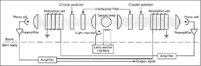
Legend to Figure 9: The loop, composed of absorption cells, photocells, and amplifiers oscillates at a frequency proportional to the ambient field magnitude.

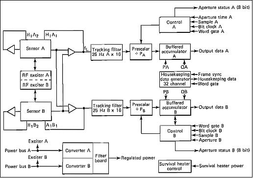
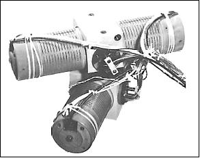
Legend to Figure 11: Each cylinder contains optics and hybrid preamplifiers for one dual cell magnetometer. The central yoke is made of beryllium to minimize the temperature gradient. A flat beryllium radiator (not shown) is attached to the top of the yoke. The entire structure is housed in a fiberglass and multilayer thermal blanket enclosure.

Vector Magnetometer

PI: Mario H. Acuna, GSFC, fluxgate type, with an accuracy of < 3 nT for each component <3 nT (after in-flight calibration). The fluxgate magnetometer was a a state-of-the-art instrument that covered the range of ±64,000 nT (nanoTesla) using a ±2000 nT basic magnetometer and digitally controlled current sources to increase its dynamic range. The instrument consisted of three fluxgate ring-core sensors mounted on a MACOR (machinable ceramic) structure. ^{16) 17)}

The on-board attitude determination system required two star cameras, two ATS (Attitude Transfer System) optical heads (for pitch/yaw and roll). Two ATS (pitch/yaw and roll) mirrors were mounted on the back of the vector magnetometer at the end of the boom, providing a reflected beam of light for accurate magnetometer axis determination. A precision sun sensor was mounted in addition on the vector magnetometer for redundant measurements.

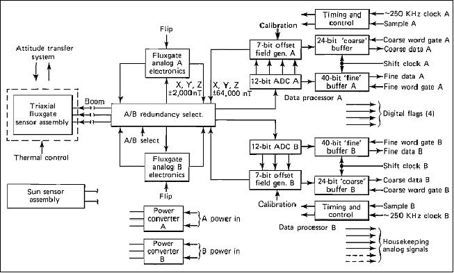
As can be seen from Figure 12, the magnetometer electronics, analog-to-digital converters, and digitally controlled current sources were implemented with redundant designs. This was also true for the digital processors and power converters. The block-redundancy approach provided a fundamental measure of reliability to this important instrument and eliminated from consideration single-point failures in the electronics. Selection of the particular system used (A or B in Figure 12) for both the analog and digital portions of the instrument was executed by ground command.

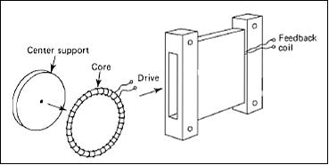
The instrument design took advantage of the ring core geometry. This particular geometry exhibits superior performance characteristics in terms of noise and zero-level stability. In addition, its uniform expansion characteristics were essential for achieving the angular stability required. Figure 13 is a schematic diagram that shows the construction of each sensor (all parts have identical expansion coefficients). Crucial elements in the Magsat fluxgate sensor design were the feedback coil that nulls the external field , and the sensor core itself; they constitute the most important sources of error in terms of alignment stability as well as variation of scale factor with temperature. Any distortion or motion of the sensor core within the feedback coil represents an effective alignment shift. Structural deformations of > 50 µm were sufficient to exceed the alignment stability tolerance.

The electronics design for the vector magnetometer incorporated a number of advanced developments derived from the Voyager 1 and 2 magnetic field experiments that were directly applicable to this instrument. However, the extreme accuracy required of the analog signal processing circuits dictated the use of ultra-precise components, some of which had to be specifically developed for Magsat. The maximum allowable error voltage for the digitally controlled current sources was only 125 µV, so considerable attention had to be paid to the problem of thermally generated electromotive forces that are produced across dissimilar metal junctions.

Calibration and alignment: The problem of determining the orientation of a given magnetic field vector traditionally has been solved by assuming that the field orientation can be established accurately by the geometry of a calibration coil. This method is generally sufficient to determine sensor orientation within a few arcminutes from its true direction, but it is certainly not accurate enough for the MagSat case where accuracies of the order of 2 arcsec were required. The method to determine the sensor alignment assumed that the deviations from orthogonality of the sensor assembly and triaxial test coil system were small. In this case, a very accurate alignment of the sensor and test coil system can be obtained simultaneously by rotating the sensor twice through exactly 90° in two planes.

An accurate optical reference coordinate system was first established at Magnetics Test Facility of GSFC by means of a pair of first-order theodolites referenced to a 400 m baseline. Numerous magnetic contamination problems associated with the optical system had to be solved to realize the intrinsic accuracy obtainable by this method. The short- and long-term mechanical stability of the triaxial coil system presented very difficult problems at times in terms of the consistency of test results. Nevertheless, after many hours of dedicated testing to determine the true performance of the magnetometer and coil system, excellent results were obtained, as is evident by the outstanding in-orbit performance of the vector magnetometer.

Data: MagSat carried two on-board tape recorders to allow 10 hours of recorded data to be dumped to a NASA ground station during a pass. The data are available in several formats from the National Space Science Data Center (NSSDC) at GSFC and at NOAA/ NGDC (subset of NASA data). ¹⁸⁾

References

1) ”Johns Hopkins APL Technical Digest, Vol. 1, No 3, July-Sept. 1980, Special Issue of MagSat, URL: http://core2.gsfc.nasa.gov/research/mag_field/purucker/APL-Technical-Digest_1-3.pdf

2) F. Mobley, L. Eckard, G. Fountain, G. Ousley, “MAGSAT--A new satellite to survey the earth's magnetic field,” IEEE Transactions on Magnetics, Vol. 16, Issue 5, Sept. 1980, pp. 758-760

3) Space Applications, Vol. 6, Chapter 2, “NASA Historical Data Book,” URL: http://history.nasa.gov/SP-4012/vol6/vol_vi_ch_2.pdf MAgSat is on pp. 45-46, and in Tables 2-81 and 2-82 (pp. 125-127)

4) Gilbert W. Ousley, “Overview of the MagSat Program,” Vol. 1, No 3, July-Sept. 1980, Special Issue of MagSat, pp.171-174, URL: http://core2.gsfc.nasa.gov/research/mag_field/purucker/APL-Technical-Digest_1-3.pdf

5) F. W. Schenkel, A. Finkel, “The APL MAGSAT Attitude Transfer System Concept,” APL/JHU, CP 055, April 1977, URL: http://www.dtic.mil/cgi-bin/GetTRDoc?AD=ADA040987

6) K. J. Heffernan, G. H. Fountain, B. E. Tossman, F. F. Mobley, “The Magsat Attitude Control System,” JHU/APL Technical Digest, Vol. 1, No 3, July-Sept. 1980, pp. 188-193, URL: http://core2.gsfc.nasa.gov/research/mag_field/purucker/APL-Technical-Digest_1-3.pdf

7) G. H. Fountain, F. W. Schenkel, T. B. Coughlin, C. A. Wingate, “The Magsat Attitude Determination System,” JHU/APL Technical Digest, Vol. 1, No 3, July-Sept. 1980, pp. 194-200, URL: http://core2.gsfc.nasa.gov/research/mag_field/purucker/APL-Technical-Digest_1-3.pdf

8) Ark L. Lew, “The Microprocessor-based MagSat command system,” JHU-APL, CP 077, Feb. 1980, URL: http://www.retrotechnology.com/memship/magsat_command.pdf

9) J. F. Smola, “The Magsat Magnetometer Boom System,” JHU/APL Technical Digest, Vol. 1, No 3, July-Sept. 1980, pp. 2001-204

10) G. H. Fountain, F. F. Mobley, B. E. Tossman,C. E. Williams, “A sampled-data attitude-control system for the MAGSAT spacecraft,” Proceedings of the Ninth Annual Pittsburgh Conference, `Modeling and simulation,' Pittsburgh, PA., April 27-28, 1978,. Vol. 9, Part 3. (A79-23776 08-59)

11) Michael E. Purucker, “MagSat,” URL: http://core2.gsfc.nasa.gov/research/purucker/encyclopedia/magsat/MAGSAT.pdf

12) B. E. Tossman, F. F. Mobley, G. H. Fountain, K. J. Hefferman, J. C. Ray, C. E. Williams, “MAGSAT attitude control system design and performance,” Guidance and Control Conference, Danvers, MA., August 11-13, 1980, AIAA-1980-1730

13) Ark L. Lew, Bruce C. Moore, John R. Dozsa, Ronald K. Burek, “”The MagSat Telecommunications System,” JHU/APL Technical Digest, Vol. 1, No 3, July-Sept. 1980, pp. 183-187, URL: http://core2.gsfc.nasa.gov/research/mag_field/purucker/APL-Technical-Digest_1-3.pdf

14) Robert Langel. Gilbert Ousley, John Berbert, James Murphy, Mark Settle, “The MAGSAT mission,” Geophysical Research Letters, Vol. 9, No 4, 1982, pp. 243–245, doi:10.1029/GL009i004p00243

15) W. H. Farthing, “The Magsat Scalar Magnetometer,” JHU/APL Technical Digest, Vol. 1, No 3, July-Sept. 1980, pp. 205-209, URL: http://core2.gsfc.nasa.gov/research/mag_field/purucker/APL-Technical-Digest_1-3.pdf

16) M. H. Acuna, “The Magsat Precision Vector Magnetometer,” JHU/APL Technical Digest, Vol. 1, No 3, July-Sept. 1980, pp. 210-213, URL: http://core2.gsfc.nasa.gov/research/mag_field/purucker/APL-Technical-Digest_1-3.pdf

17) M. H. Acuna, C. S. Scearce, J. B. Seek, J. Schelfele, “The MAGSAT Vector Magnetometer - A Precision Fluxgate Magnetometer for the Measurement of the Geomagnetic Field,” NASA Technical Memorandum 79656, October 1978, URL: http://ia600501.us.archive.org/18/items/nasa_techdoc_19790010349/19790010349.pdf

18) Robert A. Langel, “Magsat Scientific Investigations,” JHU/APL Technical Digest, Vol. 1, No 3, July-Sept. 1980, pp. 214-227, URL: http://core2.gsfc.nasa.gov/research/mag_field/purucker/APL-Technical-Digest_1-3.pdf
 

The information compiled and edited in this article was provided by Herbert J. Kramer from his documentation of: ”Observation of the Earth and Its Environment: Survey of Missions and Sensors” (Springer Verlag) as well as many other sources after the publication of the 4th edition in 2002. - Comments and corrections to this article are always welcome for further updates (eoportal@symbios.space).