EO
ESA
Atmosphere
Ocean
Sentinel-3 (S3) is a constellation of oceanography and land monitoring satellites operated by the European Space Agency (ESA) and supported by EUMETSAT (European Organisation for the Exploitation of Meteorological Satellites). Both S3A, launched in February 2016, and S3B, launched in April 2018, are part of Copernicus - the European Union’s Earth observation program, managed by the European Commission (COM).
Quick facts
Overview
| Mission type | EO |
| Agency | ESA, EUMETSAT, COM |
| Mission status | Operational (nominal) |
| Launch date | 16 Feb 2016 |
| Measurement domain | Atmosphere, Ocean, Land, Gravity and Magnetic Fields, Snow & Ice |
| Measurement category | Cloud type, amount and cloud top temperature, Atmospheric Temperature Fields, Cloud particle properties and profile, Ocean colour/biology, Aerosols, Multi-purpose imagery (ocean), Radiation budget, Multi-purpose imagery (land), Surface temperature (land), Vegetation, Albedo and reflectance, Gravity, Magnetic and Geodynamic measurements, Surface temperature (ocean), Atmospheric Humidity Fields, Landscape topography, Ocean topography/currents, Sea ice cover, edge and thickness, Snow cover, edge and depth, Ocean surface winds, Ocean wave height and spectrum, Ice sheet topography |
| Measurement detailed | Cloud top height, Precipitation Profile (liquid or solid), Atmospheric pressure (over sea surface), Ocean imagery and water leaving spectral radiance, Ocean chlorophyll concentration, Cloud cover, Cloud optical depth, Aerosol optical depth (column/profile), Cloud type, Color dissolved organic matter (CDOM), Cloud base height, Aerosol Extinction / Backscatter (column/profile), Land surface imagery, Aerosol effective radius (column/profile), Fire temperature, Vegetation type, Fire fractional cover, Earth surface albedo, Leaf Area Index (LAI), Land cover, Atmospheric specific humidity (column/profile), Land surface temperature, Sea surface temperature, Land surface topography, Ocean suspended sediment concentration, Sea-ice cover, Snow cover, Wind speed over sea surface (horizontal), Cloud top temperature, Normalized Differential Vegetation Index (NDVI), Sea-ice thickness, Volcanic ash, Significant wave height, Photosynthetically Active Radiation (PAR), Geoid, Fraction of Absorbed PAR (FAPAR), Sea level, Ocean dynamic topography, Sea-ice sheet topography, Sea-ice surface temperature, Atmospheric pressure (over land surface), Diffuse attenuation coefficient (DAC), Short-wave cloud reflectance |
| Instruments | OLCI, SRAL, SLSTR, DGXX-S |
| Instrument type | Imaging multi-spectral radiometers (vis/IR), Precision orbit, Radar altimeters |
Related Resources
Summary
Mission Capabilities
The S3 satellites measure sea-surface topography, as well as the colour and temperature of ocean and land surfaces. This data is used for ocean systems forecasting, environmental monitoring, and climate monitoring.
Both satellites are identical and have three instruments on board: an imaging multispectral radiometer and ocean colour instrument - the Ocean and Land Colour Imager (OLCI); another imaging radiometer - the Sea and Land Surface Temperature Radiometer (SLSTR); and a radar altimeter - the SAR (Synthetic Aperture Radar) Radar Altimeter (SRAL), which is complemented by a Microwave Radiometer (MWR). MWR complements SRAL by monitoring the water vapour and cloud water contents in its field of view to enable data correction.
Performance Specifications
OLCI has 21 spectral bands ranging over VNIR (visual and near-infrared) and SWIR (short-wave infrared), with a spatial resolution of 300 m for all bands and a swath of 1270 km. The division of the field of view between five cameras allows for such a large swath. OLCI is angled 12.2° away from the sun to minimise the effect of sunglint. SLSTR has 11 spectral bands: the VNIR and SWIR channels have three bands each with a resolution of 500 m, and the MWIR (medium wave infrared) and TIR (thermal infrared) channels cover five bands with a spatial resolution of 1 km. When observing nadir, SLSTR has a swath of 1420 km and when facing backwards has a swath of 750 km. SRAL operates in both C-band and Ku-band with a resolution of 300 m, while MWR operates in both K-band and Ka-band.
The two S3 satellites follow the same sun-synchronous orbit with an inclination of 98.65° but are 180° out of phase. They orbit at an altitude of 807 km with a period of 101 minutes. The revisit time is less than or equal to four days (varies with latitude), with the cycle repeating every 27 days.
Space and Hardware Components
The other key instrument onboard is the Precise Orbit Determination (POD) package, consisting of a Global Navigation Satellite Systems (GNSS) receiver, a Doppler Orbit determination and Radio-positioning Integrated on Satellite (DORIS) instrument, as well as a Laser Retro-Reflector (LRR). The GNSS receiver contributes to satellite control and accurate onboard timing; the DORIS is a precise satellite tracking system that uses the Doppler effect and the exact position of the satellite to calculate the satellite's orbit; while the LRR reflects any laser pulses sent from ground stations so they can accurately measure their distance from the satellite.
S3C and S3D are expected to launch in 2024 and 2028 respectively to provide continuity to the S3 missions after S3A and S3B reach their end of life, expected in 2026 and 2028 respectively.
Copernicus: Sentinel-3 — Global Sea/Land Monitoring Mission including Altimetry
Spacecraft Launch Mission Status Sensor Complement Ground Segment References
The Sentinel-3 (S3) mission of ESA and the EC is one of the elements of the GMES (Global Monitoring for Environment and Security) program, which responds to the requirements for operational and near-real-time monitoring of ocean, land and ice surfaces over a period of 20 years. The topography element of this mission will serve primarily the marine operational users but will also allow the monitoring of sea ice and land ice, as well as inland water surfaces, using novel observation techniques.The Sentinel-3 mission is designed as a constellation of two identical polar orbiting satellites, separated by 180º, for the provision of long-term operational marine and land monitoring services. The operational character of this mission implies a high level of availability of the data products and fast delivery time, which have been important design drivers for the mission. 1) 2) 3) 4) 5) 6) 7) 8) 9) 10) 11) 12) 13) 14)
The Sentinel-3 program represents a series of operational spacecraft over the envisioned service period to guarantee access to an uninterrupted flow of robust global data products.
Copernicus is the new name of the former GMES program 15)
Copernicus is the new name of the European Commission's Earth Observation Programme, previously known as GMES (Global Monitoring for Environment and Security). The new name was announced on December 11, 2012, by EC (European Commission) Vice-President Antonio Tajani during the Competitiveness Council.
In the words of Antonio Tajani: “By changing the name from GMES to Copernicus, we are paying homage to a great European scientist and observer: Nicolaus Copernicus (1473-1543). As he was the catalyst in the 16th century to better understand our world, so the European Earth Observation Programme gives us a thorough understanding of our changing planet, enabling concrete actions to improve the quality of life of the citizens. Copernicus has now reached maturity as a programme and all its services will enter soon into the operational phase. Thanks to greater data availability user take-up will increase, thus contributing to that growth that we so dearly need today.”
The main observation objectives of the mission are summarised in the following list:
• Ocean and land colour observation data, free from sun-glint, shall have a revisit time of 4 days (2 days goal) and a quality at least equivalent to that of Meris instrument on Envisat. The actual revisit obtained over ocean at the equator (worst case) is less than 3.8 days with a single satellite and drops below 1.9 days with 2 satellites, phased 180° on the same orbital plane.
• Ocean and land surface temperature shall be acquired with at least the level of quality of AATSR on Envisat, and shall have a maximum revisit time of 4 days with dual view (high accuracy) observations and 1 day with single view. Achieved performance is shown to be significantly better, even with a single satellite (dual view: 3.5 days max, 1.8 days average).
• Surface topography observations shall primarily cover the global ocean and provide sea surface height (SSH) and significant wave height (SWH) to an accuracy and precision at least equivalent to that of RA-2 on Envisat. Additionally, Sentinel-3 shall provide surface elevation measurements -in continuity to CryoSat-2 - over ice regions covered by the selected orbit, as well as measurements of in-land water surfaces (rivers and lakes).
In addition, Sentinel-3 will provide surface vegetation products derived from synergistic and co-located measurements of optical instruments, similar to those obtained from the Vegetation instrument on SPOT, and with complete Earth coverage in 1 to 2 days.
The EU Marine Core Service (MCS) and the Land Monitoring Core Service (LMCS), together with the ESA GMES Service Element (GSE), have been consolidating those services where continuity and success depends on operational data flowing from the Sentinels.
The operational character of the mission implies a high level of availability of the data products and fast delivery time, which have been important design drivers for the mission.
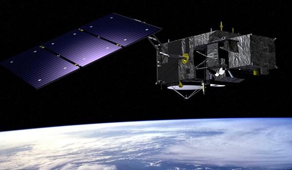
Legend to Figure 1: Sentinel-3 is arguably the most comprehensive of all the Sentinel missions for Europe’s Copernicus programme. Carrying a suite of state-of-the-art instruments, it provides systematic measurements of Earth’s oceans, land, ice and atmosphere to monitor and understand large-scale global dynamics and provide critical information for ocean and weather forecasting.
Spacecraft
The Sentinel-3 spacecraft is being built by TAS-F (Thales Alenia Space-France). A contract to this effect was signed on April 14, 2008. The spacecraft is 3-axis stabilised, with nominal pointing towards the local normal and yaw steering to compensate for the Earth rotation affecting the optical observations. The spacecraft has a launch mass of about 1150 kg, the height dimension is about 3.9 m. The overall power consumption is 1100 W. The design life is 7.5 years, with ~100 kg of hydrazine propellant for 12 years of operations, including deorbiting at the end.
AOCS (Attitude and Orbit Control Subsystem): The spacecraft is 3-axis stabilised based on the new generation of avionics for the TAS-F LEO (Low Earth Orbit) platform. The AOCS software of the GMES/Sentinel-3 project is of PROBA program heritage. NGC Aerospace Ltd (NGC) of Sherbrooke, (Québec), Canada was responsible for the design, implementation and validation of the autonomous GNC (Guidance, Navigation and Control) algorithms implemented as part of the AOCS software of PROBA-1, PROBA-2, and PROBA-V. 17)
Spacecraft launch mass, design life | ~1150 kg, 7.5 years (fuel for additional 5 years) |
Spacecraft bus dimensions | 3.9 m (height) x 2.2 m x 2.21 m |
Spacecraft structure | Build around a CFRP (Carbon Fiber Reinforced Plastics) central tube and shear webs |
AOCS (Attitude and Orbit Control Subsystem) | - 3 axis stabilisation |
Pointing type | Geodetic + yaw steering |
Absolute pointing error | < 0.1º |
Thermal control | - Passive control with SSM radiators |
EPS (Electrical Power Subsystem) | - Unregulated power bus, with a Li-ion battery and GaAs solar array. |
Mechanisms | - Stepper motor SADM (Solar Array Drive Mechanism) |
Propulsion | - Monopropellant (hydrazine) operating in blow-down mode |
Data handling and software | Centralised SMU running applications for all spacecraft subsystems processing tasks, complemented by a PDHU (Payload Data Handling Unit) for instruments data acquisition and formatting before transmission to the ground segment. |
Operational autonomy | 27 days |
Data handling architecture: The requirements for the Sentinel-3 data handling architecture call for: a) minimised development risks, b) system at minimum cost, c) operational system over 20 years. This has led to design architecture as robust as possible using a single SMU (Satellite Management Unit) computer as the platform controller, a single PDHU (Payload Data-Handling Unit) for mission data management, and to reuse existing qualified heritage. 18)
The payload accommodates 6 instruments, sources of mission data. The 3 high rate instruments provide mission data directly collected through the SpaceWire network, while the low rate instruments are acquired by the central computer for distribution through the SpaceWire network to the mass memory. The PDHU acquires and stores all mission data for latter multiplexing, formatting, encryption and encoding for download to the ground.
The payload architecture is built-up over a SpaceWire network (Figure 2) for direct collection of high rate SLSTR, OLCI and SRAL instruments and indirect collection of low rate MWR, GNSS and DORIS instrument data plus house-keeping data through the Mil-Std-1553 bus by the SMU, all data being acquired from SpaceWire links and managed by the PDHU.
The mission data budget is easily accommodated thanks to the SpaceWire performance. Each SpaceWire link being dedicated to point-to-point communication without interaction on the other links (no routing), the frequency is set according to the need plus a significant margin. The PDHU is able to handle the 4 SpaceWire sources at up to 100 Mbit/s.
All mission data sources (OLCI, SLSTR, SRAL and SMU) provide data through two cold redundant interfaces and harnesses. The PDHU, being critical as the central point of the mission data management, implements a full cross-strapping between nominal and redundant sources interfaces and its nominal and redundant sides.
The PDHU SpaceWire interfaces are performed thanks to a specific FPGA, the instrument’s ones are based on the ESA Atmel SMCS-332, while the SMU interfaces are implemented by an EPICA ASIC circuit developed by Thales Alenia Space.
RF communications: The S-band is used for TT&C transmissions The S-band downlink rate is 123 kbit/s or 2 Mbit/s, the uplink data rate is 64 kbit/s. The X-band provide the payload data downlink at a rate of 520 Mbit/s. An onboard data storage capacity of 300 Gbit (EOL) is provided for payload data.
Four categories of data products will be delivered: ocean colour, surface topography, surface temperature (land and sea) and land. The surface topography products will be delivered with three timeliness levels: NRT (Near-Real Time, 3 hours), STC (Standard Time Critical, 1-2 days) and NTC (Non-Time Critical, 1 month). Slower products allow more accurate processing and better quality. NRT products are ingested into numerical weather prediction and seastate prediction models for quick, short term forecasts. STC products are ingested into ocean models for accurate present state estimates and forecasts. NTC products are used in all high-precision climatological applications, such as sealevel estimates.
The resulting analysis and forecast products and predictions from ocean and atmosphere adding data from other missions and in situ observations, are the key products delivered to users. They provide a robust basis for downstream value-added products and specialised user services.
Introduction of new technology: A newly developed MEMS rate sensor (gyroscope), under the name of SiREUS, will be demonstrated on the AOCS of Sentinel-3. The gyros will be used for identifying satellite motion and also to place it into a preset attitude in association with optical sensors after its separation from the launcher, for Sun and Earth acquisition. Three of the devices will fly inside an integrated gyro unit, each measuring a different axis of motion, with a backup unit ensuring system redundancy. Each unit measures 11 cm x 11 cm x 7 cm, with an overall mass of 750 grams. 19)
The SiREUS device is of SiRRS-01 heritage, a single-axis rate sensor built by AIS (Atlantic Inertial Systems Ltd., UK), which is using a ’vibrating structure gyro’, with a silicon ring fixed to a silicon structure and set vibrating by a small electric current. The SiRRS-01 MEMS gyro has been used in the automobile industry. These devices are embedded throughout modern cars: MEMS accelerometers trigger airbags, MEMS pressure sensors check tires and MEMS gyros help to prevent brakes locking and maintain traction during skids. - In a special project, ESA selected the silicon-based SiRRS-01 to have it modified for space use (and under the new name of SiREUS).
Development Status
• May 04, 2020: During these unprecedented times of the COVID-19 lockdown, trying to work poses huge challenges for us all. For those that can, remote working is now pretty much the norm, but this is obviously not possible for everybody. One might assume that like many industries, the construction and testing of satellites has been put on hold, but engineers and scientists are finding ways of continuing to prepare Europe’s upcoming satellite missions such as the next Copernicus Sentinels. 21)
- Despite COVID-19, a milestone has been reached for the Copernicus Sentinel-3 mission, with the transport of the ‘D’ satellite platform from Thales Alenia Space in Rome, Italy, to Cannes in France.
- There are currently two Sentinel-3 satellites in orbit: Sentinel-3A and Sentinel-3B. They work as a pair to measure systematically Earth’s oceans, land, ice and atmosphere to monitor and understand large-scale global dynamics, and to provide essential information in near-real time for ocean and weather forecasting.
- To ensure continuity, they will eventually be replaced by Sentinel-3C and Sentinel-3D. Therefore, work is ongoing to prepare these next satellites.
- Nic Mardle, ESA’s Copernicus Sentinel-3 project manager, said, “At the start of the restrictions the Thales team in Italy worked particularly hard to try to complete everything for Sentinel-3D before a full lockdown was imposed. Single shifts with no hand-over allowed two teams to continue working on the satellite with no risk of infecting each other.
- “They were almost complete when the full shutdown of the facilities was announced, but this did not stop the Thales teams in Italy and in France and us at ESA, as we all continued by working remotely to get though the all-important ‘Delivery Review Board’.
- As soon as Thales’ facilities could be accessed again, the teams completed the few final activities including the packing and shipment preparations and finalised the necessary approvals from Italian and French governments, so that the satellite platform could be transported by road from Italy to France.
- Sentinel-3D arrived safely at the Cannes facilities in the night of 21 April and was unpacked by the Thales-Alenia Cannes team with the remote support from their colleagues in Rome.
- Nic added, “Activities are definitely more complicated in this period, but all teams are working together to facilitate the continuation of the program in the most efficient and pragmatic way, finding solutions to the new problems caused by the impacts the virus, while ensuring that the health and safety of the teams involved is ensured.”
- Josef Aschbacher, ESA’s Director of Earth Observation Programs, noted, “Everybody is working under extremely difficult circumstances and I’m really happy to see that work continues to prepare numerous new missions.
- “This is not only vital to ensure the continuity of measurements of our planet from space to understand and monitor environmental changes that are affecting society worldwide, but also we need to keep demonstrating new space technologies for the future. And, with COVID-19 affecting the economy so badly, we are making every effort to keep the space industry and downstream ventures in business.”
• April 13, 2018: The team of propulsion experts has spent two days carrying out the tricky task of fuelling the Copernicus Sentinel-3B satellite with 130 kg of hydrazine and pressurising the tank for its life in orbit. 22) 23)
- Since hydrazine is extremely toxic, only specialists remained in the cleanroom for the duration. A doctor and security staff waited nearby with an ambulance and fire engine ready to respond to any problems.
- The satellite is scheduled for liftoff on 25 April from Russia’s Plesetsk Cosmodrome at 17:57 GMT (19:57 CEST).
- In orbit it will join its identical twin, Sentinel-3A, which was launched in 2016. This pairing of satellites provides the best coverage and data delivery for Copernicus.
- Sentinel-3B is the seventh Sentinel satellite to be launched for Copernicus. Its launch will complete the constellation of the first set of Sentinel missions for Europe’s Copernicus program.
• March 23, 2018: With the Sentinel-3B satellite now at the Plesetsk launch site in Russia and liftoff set for 25 April, engineers are steaming ahead with the task of getting Europe’s next Copernicus satellite ready for its journey into orbit. 24)
- After arriving at the launch site on 18 March, the satellite has been taken out of its transport container and is being set up for testing. Kristof Gantois, ESA’s Sentinel-3 engineering manager, said, “The satellite’s journey from France was hampered slightly by the freezing winter weather here in Russia, but it’s now safe in the milder cleanroom environment.
- Sentinel-3B will join its twin, Sentinel-3A, in orbit. The pairing of identical satellites provides the best coverage and data delivery for Europe’s Copernicus program – the largest environmental monitoring program in the world.
• February 2, 2018: After being put through its paces to make sure it is fit for life in orbit around Earth, the Copernicus Sentinel-3B satellite is ready to be packed up and shipped to Russia for liftoff. 25)
- Its twin, Sentinel-3A, has been in orbit since February 2016, systematically measuring our oceans, land, ice and atmosphere. The information feeds a range of practical applications and is used for monitoring and understanding large-scale global dynamics.
- The pairing of identical satellites provides the best coverage and data delivery for Europe’s Copernicus program – the largest environmental monitoring program in the world.
- Sentinel-3B has spent the last year at Thales Alenia Space’s premises in Cannes, France, being assembled and tested, and now it is fit and ready for its journey to the Plesetsk launch site in northern Russia.
- This included putting it in a vacuum chamber, exposing it to extreme temperatures, and we have also simulated the vibrations it will be subjected to during launch. - With liftoff expected to be confirmed for the end of April, the satellite will start its journey to Russia in March.
- Both Sentinel-3 satellites carry a suite of cutting-edge instruments to supply a new generation of data products, which are particularly useful for marine applications. For example, they monitor ocean-surface temperatures for ocean and weather forecasting services, aquatic biological productivity, ocean pollution and sea-level change. — Sentinel-3B also marks a milestone in Europe’s Copernicus program.
- With the Sentinel-1 and Sentinel-2 pairs already in orbit monitoring our environment, the launch of Sentinel-3B means that three mission constellations will be complete. In addition, Sentinel-5P, a single-satellite mission to monitor air pollution, has been in orbit since October 2017.
- While the Sentinel-1 and Sentinel-2 satellites circle Earth 180° apart, the configuration for Sentinel-3 will be slightly different: the 140° separation will help to measure ocean features such as eddies as accurately as possible.
- Prior to this, however, they will fly just 223 km apart, which means that Sentinel-3B will be a mere 30 seconds behind Sentinel-3A.
- Flying in tandem like this for around four months is designed to understand any subtle differences between the two sets of instruments – measurements should be almost the same given their brief separation.
- ESA’s ocean scientist, Craig Donlon, explains, “Our Sentinel-3 ocean climate record will eventually be derived from four satellites because we will be launching two further Sentinel-3s in the future.
- “We need to understand the small differences between each successive satellite instrument as these influence our ability to determine accurate climate trends. The Sentinel-3 tandem phase is a fantastic opportunity to do this and will provide results so that climate scientists can use all Sentinel-3 data with confidence.”
• December 5, 2017: EUMETSAT has confirmed the readiness of its teams and the new version of its ground segment to support the launch and commissioning of the Copernicus Sentinel-3B satellite in a two-satellite configuration with Sentinel-3A. 26)
- The new version of the ground segment includes enhancements and upgrades necessary to exploit a dual Sentinel-3 system. Its acceptance follows a comprehensive campaign of verification and validation tests.
- During the commissioning of Sentinel-3B, the two Sentinel-3 satellites will fly in close formation, 30 seconds apart. In this phase, ESA will manage Sentinel-3B flight operations, and EUMETSAT will be progressively ramping up its flight control activity to prepare the hand-over, while continuing to perform flight operations of Sentinel-3A.
- The close formation flight will allow to compare thoroughly the measurements from all instruments aboard Sentinel-3A and –B, ensuring the best consistency between the products from the two satellites.
- The completion of commissioning will lead to a handover of the Sentinel-3B satellite from ESA to EUMETSAT once the latter has been moved to it final orbital position, at a 140º phasing from Sentinel-3A, to form the full Sentinel-3 constellation. The 140° phasing was chosen to optimise global coverage and ensure optimised sampling of ocean currents by the combined altimeters on board Sentinel-3A and -3B.
- Thus the Sentinel-3 constellation will also realise the best possible synergy with the cooperative Jason-3 high precision ocean altimeter mission, another Copernicus marine and climate mission exploited by EUMETSAT on behalf of the European Union.
- Under the Copernicus data policy, all Sentinel-3 marine data and products are available on a full, free and open basis to all users through EUMETSAT’s Near Real Time dissemination channels EUMETCast, the Copernicus Online Data Access and EUMETview.
• June 1, 2017: While the Copernicus Sentinel-3A satellite is in orbit delivering a wealth of information about our home planet, engineers are putting its twin, Sentinel-3B satellite through a series of vigorous tests before it is shipped to the launch site next year. It is now in the thermal–vacuum chamber at Thales Alenia Space’s facilities in Cannes, France. This huge chamber simulates the huge swings in temperature facing the satellite in space. Once this is over, the satellite will be put through other tests to prepare it for liftoff in the spring 2018. Both Sentinel-3 satellites carry the same suite of cutting-edge instruments to measure oceans, land, ice and atmosphere. 27)
• January 14, 2016: Following the Christmas break, the Sentinel-3A satellite has been taken out of its storage container and woken up as the campaign to prepare it for launch resumes at the Russian Plesetsk Cosmodrome. Liftoff is set for 4 February. 28)
• Nov. 20, 2015: The Sentinel-3A spacecraft has left France bound for the Plesetsk launch site in Russia and launch in late December. An Antonov aircraft carries the precious cargo to Arkhangelsk in Russia after a stopover in Moscow to clear paperwork. 29)
• Oct. 15, 2015: Before the latest satellite for Copernicus is packed up and shipped to the Plesetsk Cosmodrome in Russia for launch at the end of the year, the media and specialists were given the chance to see this next-generation mission center-stage in the cleanroom. The event was hosted by Thales Alenia Space in Cannes, France, where engineers have spent the last few years building and testing Sentinel-3A. 30)
• In December 2014, the Sentinel-3A spacecraft is now fully integrated, hosting a package of different instruments to monitor Earth’s oceans and land. After spending many months carefully piecing the satellite together, it is now being tested in preparation for launch towards the end of 2015. 31)
- Environmental tests will start in early 2015.
• In July 2014, the OLCI instrument was delivered and mounted onto the satellite.
Launch: The Sentinel-3A spacecraft was launched on February 16, 2016 (17.57 GMT) on a Rockot/Briz-KM vehicle of Eurockot Launch Services (a joint venture between Astrium, Bremen and the Khrunichev Space Center, Moscow). The launch site was the Plesetsk Cosmodrome in northern Russia. The satellite separated 79 minutes into the flight. 32) 33)
ESA awarded the contract to Eurockot Launch Services on Feb. 9, 2012. 34)
There are three spacecraft in this series: Sentinel-3A, -3B, and -3C. The second satellite is expected to be launched ~18 months after the first one.
Orbit: Frozen sun-synchronous orbit (14 +7/27 rev./day), mean altitude = 815 km, inclination = 98.6º, LTDN (Local Time on Descending Node) is at 10:00 hours. The revisit time is 27 days providing a global coverage of topography data at mesoscale.
With 1 satellite, the ground inter-track spacing at the equator is 2810 km after 1 day, 750 km after four days, and 104 km after 27 days.
For the altimetry mission, simulations show that this orbit provides an optimal compromise between spatial and temporal sampling for capturing mesoscale ocean structures, offering an improvement on SSH mapping error of up to 44% over Jason - due to improved spatial sampling - and 8% over the Envisat 35-day orbit - due to better temporal sampling. After a complete cycle, the track spacing at the equator is approximately 100 km.
The Sentinel-3 mission poses the most demanding POD (Precise Orbit Determination) requirements, specially in the radial component, not only in post-processing on-ground, but also in real-time. This level of accuracy requires dual-frequency receivers. The main objective of the mission is the observation with a radar altimeter of sea surface topography and sea ice measurements (see columns 3, 4, 5 in Table 2).
Targets | Real-time | < 3 hours | < 1-3 days | < 1 month |
Radial orbit error (rms) | < 3 m | < 8 cm | < 3 cm | < 2 cm |
Application | Support tracking mode changes | Atmospheric dynamics | Ocean | Global change |
Launch: The Sentinel-3B satellite of ESA and the EC was launched on 25 April 2018 (17:57 GMT) on a Rockot/Briz KM vehicle of Eurockot from the Plesetsk Cosmodrome, Russia. 36) 37)
The second satellite will be placed in the same orbit with an offset of 140º; this phasing improves interleave between S-3A and S-3B for better SRAL meso-scale sampling of 4-7 days. 38)
Commissioning will include a 4-5 month tandem flight. A tandem phase operation of the A/B pair with ~30 s separation in time between satellites on near identical ground-track for ~4-5 months will be flown during Phase E1.
With two satellites flying simultaneously, the following coverage will be achieved (Ref. 11):
- Global Ocean colour data is recorded with OLCI and SLSTR in less than 1.9 days at the equator, and in less than 1.4 days at latitudes higher than 30º, ignoring cloud effects.
- Global Land colour data is recorded with OLCI and SLSTR in less than 1.1 days at the equator, and less than 0.9 days in latitudes higher than 30º.
- Global Surface temperature data is recorded in less than 0.9 days at the equator and in less than 0.8 days in latitudes higher than 30º.
- Continuous altimetry observations where global coverage is achieved after completion of the reference ground track of 27 days.
Note: As of May 2020, the previously single large Sentinel-3 file has been split into three files, to make the file handling manageable for all parties concerned, in particular for the user community.
• This article covers the Sentinel-3 mission and its imagery in the period 2020-2022
• Sentinel-3 mission and its imagery in the period 2019
• Sentinel-3 imagery in the period 2018-2016
Mission Status (2021-2022)
• July 20, 2022: With searing temperatures and a string of record highs being smashed across western Europe, the current heatwave is all too apparent. Extreme heat warnings have been issued in several countries including France, Spain and Portugal, and deadly wildfires have forced thousands to flee their homes. The satellite images here are an example of how the crisis is being viewed by satellites orbiting Earth. 39)
- As the image of Figure 12 clearly shows, in some places the surface of the land reached 55°C. Considering Copernicus Sentinel-3 acquired these data in the morning, the temperature would have increased through the afternoon. Scientists monitor land-surface temperature because the warmth rising from Earth’s surface influences weather and climate patterns. These measurements are also particularly important for farmers evaluating how much water their crops need and for urban planners looking to improve heat mitigating strategies, for example. The Copernicus Emergency Management Service was activated to respond to many of the fires that are plaguing Europe at the moment, including those impacting Gironde.
• July 01, 2022: The Copernicus Sentinel-3 mission captured this impressive, wide-angled view of Patagonia at the southern end of South America, as well as the Falkland Islands (Malvinas). 40) Patagonia, a region of 673,000 km2, is divided by Argentina and Chile and includes the Andes Mountains. It includes the island archipelago of Tierra del Fuego, which is shared by Argentina and Chile. The Strait of Magellan connects the region to mainland Argentina. Alberto de Agostini National Park, a UNESCO Biosphere Reserve, features an irregular coastline and tidewater glaciers. The Falkland Islands, located 600 km east of Patagonia, are located in the South Atlantic Ocean. The region is home to densely concentrated phytoplankton blooms, which thrive in nutrient-rich waters. Copernicus Sentinel-3, a suite of instruments, monitors Earth's oceans, land, ice, and atmosphere to understand large-scale global dynamics.
• May 25, 2022: For the first time ever recorded, in the late summer of 2021, rain fell on the high central region of the Greenland ice sheet. This extraordinary event was followed by the surface snow and ice melting rapidly. Researchers now understand exactly what went on in those fateful summer days and what we can learn from it. 41) The upper-most parts of Greenland’s enormous ice cap used to be too cold for anything other than snow to fall, but not anymore. Researchers from the Department of Glaciology and Climate at the Geological Survey of Denmark and Greenland (GEUS) in collaboration with colleagues from France and Switzerland have scrutinised these questions and come up with the answers. It didn’t only rain at Summit Camp – rain was measured by new automatic weather stations placed across the ice sheet by GEUS’ ice-sheet monitoring projects PROMICE and GC-Net.
- Studying detailed data from these stations alongside measurements of surface reflectivity, or albedo, from the Copernicus Sentinel-3 satellite mission and information on atmospheric circulation patterns, the researchers discovered that the rain had been preceded by a heatwave at a time of year when seasonal melting is usually slowing down. In fact, this sudden increase of surface ice melt on Greenland could have happened without any rain ever touching the ground. The main culprit was the heat itself, melting and completely removing the surface snow, thereby changing the surface albedo, Greek for ‘whiteness’, so that Greenland snow and ice absorbed more of the Sun’s rays. The researchers found that, between 19 and 20 August 2021, this melt caused the altitude of the ice sheet’s snowline near Kangerlussuaq to retreat in elevation by a whopping 788 metres, the snowline retreated, exposing a wide area of dark bare ice.
• April 29, 2022: India is was facing a prolonged heatwave, with temperatures exceeding 42°C in numerous cities across the country. This comes just weeks after India recorded its hottest March since the country’s meteorological department began its records over 120 years ago. This image, produced using data from the Copernicus Sentinel-3 mission, shows the land surface temperature across most of the nation. 42)
- According to the India Meteorological Department, maximum air temperatures reached 43-46°C over most parts of Rajasthan, Vidarbha, Madhya Pradesh and East Uttar Pradesh; in many parts over Gujarat, interior Odisha; and in some parts of Madhya Maharashtra on 28 April. Forecasters warned that heatwave conditions are expected to continue until 2 May. Experts at the Indian Institute of Technology’s Water and Climate Lab stated that, in recent years, the number of Indian states hit by heatwaves has increased, as extreme temperatures become more frequent. Owing to the absence of cloud cover on 29 April (10:30 local time), the Sentinel-3 mission was able to obtain an accurate measurement of the land surface temperature of the ground, which exceeded 60°C in several areas. The data shows that surface temperature in Jaipur and Ahmedabad reached 47°C, while the hottest temperatures recorded are southeast and southwest of Ahmedabad (visible in deep red) with maximum land surface temperatures of around 65°C.
• April 15, 2022: The Scandinavian Peninsula, which comprises Sweden and Norway, is approximately 1850 km long. It extends southward from the Barents Sea in the north, the Norwegian sea to the west and the Gulf of Bothnia and the Baltic Sea to the east. Denmark, Finland, Latvia and Lithuania are also visible in this week’s image. 43) Along the left side of the peninsula, the jagged fjords lining Norway’s coast can be spotted from space. Many of these fjords were carved out by the thick glaciers that formed during the last ice age. The largest and deepest fjord on Norway’s coast, called Sognefjord, lies in southwest Norway and is 1308 m deep.
- Sweden’s topography consists mainly of flat, rolling lowlands dotted with lakes. Lake Vänern and Lake Vättern, the largest lakes of Sweden, are clearly visible at the bottom of the peninsula. The lakes do not freeze completely during the winter months. To the northeast of the peninsula lies Finland with more than 55,000 lakes – most of which were also created by glacial deposits. During March, much of northern Europe and Scandinavia had been affected by a strong high-pressure weather system, which also allowed for this almost cloud-free acquisition. On 19 March in Tirstrup, Denmark, the atmospheric pressure reached 1051.6 hPa, the highest value ever recorded in March.
• January 20, 2022: In July 2017, a giant iceberg, named A-68, snapped off Antarctica’s Larsen-C ice shelf and began an epic journey across the Southern Ocean. Three and a half years later, the main part of iceberg, A-68A, drifted worryingly close to South Georgia. Concerns were that the berg would run aground in the shallow waters offshore. This would not only cause damage to the seafloor ecosystem but also make it difficult for island wildlife, such as penguins, to make their way to the sea to feed. Using measurements from satellites, scientists have charted how A-68A shrunk towards the end of its voyage, which fortunately prevented it from getting stuck. However, the downside is that it released a colossal 152 billion tonnes of freshwater close to the island, potentially having a profound effect on the island’s marine life. 44) Antarctic iceberg A-68, once twice the size of Luxemburg, lost a chunk of ice after being calved, renaming it A-68A. Its offspring became A-68B and A-68C. A-68A initially stayed in the Weddell Sea, experiencing little melting. However, as it traveled across the Drake Passage, it began to melt, resulting in a 67-meter thickness and a sharp increase in melting rate. A paper published in Remote Sensing of Environment describes how researchers from the Centre for Polar Observation and Modelling in the UK and the British Antarctic Survey combined measurements from different satellites to chart how A-68A changed in area and thickness throughout its life cycle. 45)
- The journey of A-68A was charted using observations from five different satellite missions. To track how the area of A-68A changed, they used optical imagery from the Copernicus Sentinel-3 mission and from the MODIS instrument on the US Terra mission, along with radar data from the Copernicus Sentinel-1 mission. While the Sentinel-1 radar imagery offers all-weather capability and higher spatial resolution, MODIS and Sentinel-3 optical imagery have higher temporal resolution but cannot be used during the polar night and on cloudy days. To measure changes in the iceberg’s freeboard, or the height of the ice above the sea surface, they used data from ESA’s CryoSat mission and from the US ICESat-2 mission. Knowing the freeboard of the ice means that the thickness of the entire iceberg can be calculated.
- The new study reveals that A-68A collided only briefly with the sea floor and broke apart shortly afterwards, making it less of a risk in terms of blockage. By the time it reached the shallow waters around South Georgia, the iceberg’s keel had reduced to 141 metres below the ocean surface, shallow enough to just avoid the seabed which is around 150 metres deep. If an iceberg’s keel is too deep it can get stuck on the sea floor. This can be disruptive in many ways; the scour marks can destroy fauna, and the berg itself can block ocean currents and predator foraging routes. However, a side effect of the melting was the release of a colossal 152 billion (152 x 109) tonnes of freshwater close to the island – a disturbance that could have a profound impact on the island’s marine habitat. When icebergs detach from ice shelves, they drift with the ocean currents and wind, releasing cold fresh meltwater and nutrients as they melt. This process influences the local ocean circulation and fosters biological production around the iceberg.
• August 3, 2021: This map shows the temperature of the land surface on 2 August 2021. It is clear to see that surface temperatures in Turkey and Cyprus have reached over 50°C, again. A map we published on 2 July shows pretty much the same situation. The Mediterranean has been suffering a heatwave for some weeks, leading to numerous wildfires. Turkey, for example, is reported to be amid the country’s worst blazes in at least a decade. 46) The Copernicus Sentinel-3 satellites also captured smoke billowing from the fires in Turkey on 30 July.
• August 2, 2021: Captured by the Copernicus Sentinel-3 mission on 30 July 2021, this image shows smoke billowing from several fires along the southern coast of Turkey. Turkey has been battling deadly wildfires since last week. 47) Southeast Europe was experiencing extremely high temperatures. Greece is reported to be expecting an all-time European record today of 47°C. The heatwave, the result of a heat dome, has seen temperatures reach above 40°C in many areas, and meteorologists expect the weather will continue this week, making it the most severe heatwave since the 1980s. Fires had also been raging in Spain, Italy and Greece, some of which have led to the Copernicus Emergency Mapping Service being triggered. The mapping service uses data from satellites to aid response to disasters such as wildfires and floods.
• July 7, 2021: New ESA-funded research demonstrates how a specific way of processing satellite altimetry data now makes it possible to determine sea-level change in coastal areas with millimeter per year accuracy, and even if the sea is covered by ice. 48) A new processing technique shows regional differences in sea-level rise, revealing that between 1995 and 2019, sea levels increased by 2-3 mm in the south along German and Danish coasts and 6 mm in the northeast. The 2019 UN Intergovernmental Panel on Climate Change report predicts global mean sea levels to rise between 0.29 m and 1.1 m by the end of this century.
- Sea level rise is not at the same rate everywhere, and mapping rise nearer the coastline is more difficult due to mountains, bays, and offshore islands distorting radar signals. Researchers at the Technical University of Munich have developed algorithms to process measurement data from satellite altimetry sensors to yield precise and high-resolution measurements of sea-level changes in coastal areas and in leads between sea ice. The team developed a multi-stage process to handle hundreds of millions of radar measurements taken between 1995 and 2019. They calibrated the measurements from various satellite missions, detected signals from ice-covered seawater in radar reflections produced along cracks and fissures called leads, and achieved better resolution of radar echoes close to land. This enabled the measurement of sea level in coastal areas and comparison with local tidal records. The processed data were fitted to a fine grid with a resolution of 6-7 km, resulting in a highly precise dataset covering the entire Baltic Sea region. The sea level has risen at an annual rate of 2-3 mm in the south along the German and Danish coasts, compared to 6 mm in the northeast in the Bay of Bothnia. The Baltic SEAL dataset is available at balticseal.eu
• July 2, 2021: Scorching temperatures hit both Greece and Turkey this week, leading to the temporary closure of the Acropolis – Greece’s most visited monument. 49) This map shows the land surface temperature of Greece and surrounding countries on 30 June. The data show that surface temperatures reached over 50°C in many locations including the northwest of Athens and many regions in Turkey. The blue spots visible near Albania are clouds.
• July 1, 2021: While heatwaves are quite common during the summer months, the scorching heatwave hitting parts of western Canada and the US has been particularly devastating – with temperature records shattered and hundreds of people falling victim to the extreme heat. 50) Canada broke its temperature record for a third consecutive day: recording a whopping 49.6°C on 29 June in Lytton, a village northeast of Vancouver, in British Columbia. Portland, Oregon, also broke its all-time temperature record for three days in a row. The extent of the heatwave can be seen in the map below, which shows the land surface temperature of parts of Canada and the US on 29 June. The data show that surface temperatures in Vancouver and Portland reached 43°C, and Calgary recorded 45°C. The hottest temperatures recorded are in the state of Washington (visible in deep red) with maximum land surface temperatures of around 69°C. The persistent heat over parts of western Canada and parts of the US has been caused by a heat dome stretching from California to the Arctic. Temperatures have been easing in coastal areas, but there has been little respite for the inland regions.
• May 28, 2021: All five of North America’s Great Lakes are pictured in this spectacular image captured by the Copernicus Sentinel-3 mission: Lake Superior, Michigan, Huron, Erie, and Ontario. 51)The Great Lakes are a chain of deep freshwater lakes. With a combined area of around 244,000 km2, the lakes represent the largest surface of freshwater in the world – covering an area exceeding that of the United Kingdom. Around 100,000 years ago, a major ice sheet formed over Canada and the US, causing giant glaciers to flow into the land, creating valleys and leveling mountains. As temperatures increased, meltwater filled the holes left by the glaciers, creating thousands of lakes across central America and Canada. The Great Lakes, the largest remnants of this process, drain from west to east and empty into the Atlantic Ocean. Lake Superior is the largest and deepest, draining into Lake Huron via the St. Marys River. Lake Michigan is the second largest and is bounded by Michigan and Ontario. Lake Erie, the shallowest and southernmost, has been affected by toxic green algal blooms caused by phosphorus levels in the water. Parts of the Great Lakes typically freeze every winter. As Earth’s climate changes, rising air and water temperatures have led to less ice cover on many lakes in North America, including the Great Lakes.
• April 21, 2021: Oceans play a vital role in taking the heat out of climate change, but at a cost. New research supported by ESA and using different satellite measurements of various aspects of seawater along with measurements from ships has revealed how our ocean waters have become more acidic over the last three decades – and this is having a detrimental effect on marine life. 52)
- Oceans absorb 90% of the extra heat from greenhouse gas emissions and absorb 30% of the carbon dioxide from human activities, making seawater more acidic. Ocean acidification reduces the carbonate ions needed for calcifying organisms like shellfish and corals to build and maintain their hard shells, skeletons, and calcium carbonate structures. This can lead to shells and skeletons dissolved, posing serious consequences for marine life and potentially damaging the marine ecosystem. The health of our oceans is essential for regulating climate, aquaculture, food security, tourism, and other sectors. Monitoring changes in ocean acidification is crucial for climate and environmental policy-making and understanding the implications for marine life. Measurements of seawater pH are sparse and difficult to use, but variations in marine carbonate chemistry are closely related to temperature, salinity, and chlorophyll concentration, which can be measured by satellites with global coverage. A paper published recently in Earth System Science Data describes how scientists working in the OceanSODA project used measurements from ships and from satellites to show how ocean waters have become more acidic over the last three decades. 53)
- The team used a range of different satellite data, including sea-surface temperature data from the Sea and Land Surface Temperature Radiometer carried on the Copernicus Sentinel-3 satellites and from the Advanced Very High Resolution Radiometer carried on Europe’s MetOp satellites and on the US National Oceanic and Atmospheric Administration’s POES satellites. This dataset came through ESA’s Climate Change Initiative. Information on chlorophyll was also thanks to a multi-sensor blended dataset through ESA’s GlobColour project and included data from the OLCI (Ocean and Land Color Instrument) on the Copernicus Sentinel-3 satellites. Information on ocean salinity was realised through a climate reanalysis dataset called SODA3.
• February 11, 2021: Storm Darcy hit the Netherlands in the evening of Saturday 6 February as it pushed its way through much of northern Europe. Strong winds and bitter cold, which initiated a ‘code red’ weather warning, brought the country to an almost standstill as most public transport was cancelled the following day – by which time most of the country was under around 10 cm of snow. The snowfall also caused disruption to parts of the UK and Germany. 54) Although the snow stopped falling a day or so later, temperatures have remained below freezing, reawakening the Dutch passion for ice-skating. The Netherlands is home to the century-old ‘Elfstedentocht’, a 200-kilometer race on natural ice through 11 towns and cities in the northern province of Friesland. It was last held in 1997, but the current COVID pandemic restrictions mean that this historic race, which can attract thousands of participants and hundreds of thousands of spectators, is not permitted this year. Climate change is thought to be having an impact on the chances of conditions being right for an Elfstedentocht – the canal ice has to be at least 15 cm thick. According to the Dutch Meteorological Institute, KNMI, a century ago, there was a 20% chance every year of it being cold enough to organise the race, this has now decreased to an 8% chance. This image, showing snow cover in the Netherlands, northern France, Belgium, Luxembourg, Denmark, part of the UK and part of Germany, was captured by the mission’s ocean and land cover instrument.
• January 13, 2021: The heavy snowfall that hit Spain a few days ago still lies heavy across much of the country as this Copernicus Sentinel-3 satellite image shows. 55) Storm Filomena hit Spain over the weekend, covering a large part of the country in thick snow. Madrid one of the worst affected areas (see satellite image), was brought to a standstill with the airport having to be closed, trains cancelled and roads blocked. People in central Spain are struggling as a deep freeze follows the heavy snow. Yesterday, the temperature plunged to –25°C in Molina de Aragón and Teruel, in mountains east of Madrid – Spain's coldest night for at least 20 years.
• December 18, 2020: A large block of ice has broken off the northern tip of the A-68A iceberg as seen in new images captured by the Copernicus Sentinel-3 mission. 56) Satellite missions have been used to track the A-68A iceberg since its break off in 2017. The iceberg has drifted close to South Georgia, causing concerns about its potential grounding in shallow waters and potential threats to wildlife. New satellite images reveal that the iceberg has spun around clockwise, moving one end closer to the shelf and into shallow waters. This could have scraped the seafloor, causing an enormous block of ice to snap off the iceberg's northern tip. The new chunk, around 18 km long and 140 km2, is likely to be named A-68D by the US National Ice Center. The main A-68A iceberg is now approximately 3700 km2 with a length of around 135 km. The A-23A iceberg, currently stuck in the Weddell Sea, is now the world's largest iceberg.
• December 17, 2020: The snow-covered Alps are featured in this image captured by the Copernicus Sentinel-3 mission. 57) Just south of the Alps, the typical winter fog and haze can be seen over the Po Valley. The haze is most likely to be a mix of both fog and smog, trapped at the base of the Alps owing to both its topography and atmospheric conditions. Patches of snow can also be seen on the island of Corsica, Croatia and at the bottom of the Apennines in central Italy.
• October 30, 2020: All 1200 islands that make up the Republic of Maldives are featured in this spectacular image captured by the Copernicus Sentinel-3 mission. 58) The ocean and colour instrument onboard the Copernicus Sentinel-3 mission has a swath width of 1270 km which allows us to enjoy this wide view of the Maldive Islands and its surroundings. A popular tourist destination, the Maldives lie in the Indian Ocean, around 700 km southwest of the southernmost tip of mainland India, visible in the top-right of the image. The Maldives, a chain of small coral islands, is one of the world's most geographically dispersed countries, with over 80% of its land below one meter above mean sea level. This vulnerability makes its population of over 500,000 people highly susceptible to sea swells, storm surges, and severe weather. The Special Report on the Ocean and Cryosphere in a Changing Climate states that the global mean sea level is likely to rise to around 1 meter by the end of this century, potentially covering the majority of the nation. The Copernicus Sentinel-6 Michael Freilich satellite, scheduled for launch on 10 November, is the first of two identical satellites to provide accurate measurements of sea-level change. It will serve as a radar altimetry reference mission, continuing the long-term record of measurements of sea-surface height, allowing for further climate research and monitoring climate change effects.
• October 23, 2020: The Copernicus Sentinel-3 mission takes us over the Ganges Delta – the world’s largest river delta. 59) The Ganges Delta, covering around 100,000 km2, is a region in Bangladesh and India, primarily formed by the Ganges and Brahmaputra rivers. The river, which flows for over 2400 km from the Himalayas, deposits fertile soil and nutrients across its floodplain. The delta is largely covered by the Sundarbans swamp forest, the world's largest mangrove forest, providing a critical habitat for various species. The city of Kolkata, one of India's largest cities, is located near the Sundarbans. Dhaka, Bangladesh's capital, is located north of the Buriganga river. The delta is one of the most densely populated in the world and is highly vulnerable to climate change. Residents are at risk from catastrophic floods, intense rainfall, and accelerated sea-level rise. Asia, particularly low-lying coastal regions, is likely to experience the worst effects of sea-level rise by 2100. The Copernicus Sentinel-6 mission, set to launch next month, will play a crucial role in monitoring sea surface changes until at least 2030. The satellite, renamed in honor of former NASA Earth Science Division director Michael Freilich, has been transferred to the SpaceX Payload Processing Facility and undergone tests to ensure its safety during liftoff and orbit.
• September 22, 2020: Earth’s oceans help to slow global warming by absorbing carbon from our atmosphere – but fully observing this crucial process in the upper ocean and lower atmosphere is difficult, as measurements are taken not where it occurs, the sea surface, but several meters below. New research uses data from ESA, NASA and NOAA satellites to rectify this, and finds that far more carbon is absorbed by the oceans than previously thought. 60) Much of the carbon dioxide emitted by human activity does not stay in the atmosphere but is taken up by oceans and land vegetation – so-called ‘carbon sinks’. There are ongoing efforts to collect and compile in situ measurements of the ocean sink in the form of the SOCAT ( Surface Ocean CO2 Atlas), which contains over 28 million international observations of our oceans and coastal seas from 1957 to 2020. By delving into SOCAT’s vast database, scientists can identify how much carbon is being sucked out of the atmosphere and stored by our seas.
- By applying satellite corrections to SOCAT data from 1992 to 2018 to account for temperature differences between the surface and at a few meters’ depth, the researchers find a substantially higher ocean uptake of carbon dioxide than previously thought. They were able to do this thanks to data from a suite of satellites such as ESA’s Envisat, NOAA’s AVHRR, EUMETSAT’s MetOp series, and the Copernicus Sentinel-3 mission, firstly as part of the OceanFlux research project (part of ESA’s Science for Society program) and then continued within two EU-funded projects. The corrected figures reveal that the net flux of carbon into the oceans is underestimated by up to 0.9 Gigatons of carbon per year – a significant amount that, at times, doubles uncorrected values. The oceans’ role in capturing atmospheric carbon is being underestimated. While this may bring positive benefits in terms of reducing atmospheric warming due to climate change, as more carbon dioxide is being removed from the air, the oceans are impacted by the carbon they absorb. They become more acidic, which threatens the health of marine ecosystems and makes it increasingly difficult for ocean life to survive.
• September 18, 2020: 'Medicane' Ianos. Medicanes are similar in form to hurricanes and typhoons, but can form over cooler waters. While hurricanes move east to west, medicanes move from west to east. 62)
• September 11, 2020: The Western US states have been battling close to 100 wildfires, blanketing the majority of the west coast in smoke. Captured on 10 September, this Copernicus Sentinel-3 image shows the extent of the smoke plume which, in some areas, has caused the sky to turn orange. 63) The cities of Portland, Eureka, Eugene, San Francisco and Sacramento are all blanked in smoke. In the top of the image, the cities of Vancouver and Seattle are visible.
• August 14, 2020: The Copernicus Sentinel-3 mission shows a rare, cloud-free view of Iceland captured on 14 August 2020. 64)
• August 27, 2020: Over the past months, the Arctic has experienced alarmingly high temperatures, extreme wildfires and a significant loss of sea ice. While hot summer weather is not uncommon in the Arctic, the region is warming at two to three times the global average – impacting nature and humanity on a global scale. Observations from space offer a unique opportunity to understand the changes occurring in this remote region. 65) Wildfire smoke releases a wide range of pollutants including carbon monoxide, nitrogen oxides and solid aerosol particles. On 20 June, the Russian town of Verkhoyansk, which lies above the Arctic Circle, recorded a staggering 38°C. In June alone, the Arctic wildfires were reported to have emitted the equivalent of 56 megatons of carbon dioxide, as well as significant amounts of carbon monoxide and particulate matter. In addition, the Northern Hemisphere saw its hottest July since records began — surpassing the previous record set in 2019. Firstly, the high temperatures fuelled an outbreak of wildfires in the Arctic Circle. Images captured by the Copernicus Sentinel-3 mission show some of the fires in the Chukotka region, the most north-easterly region of Russia, on 23 June 2020.- - According to the Copernicus Climate Change Service, July 2020 was the third warmest July on record for the globe, with temperatures 0.5°C above the 1981-2010 average. Extreme air temperatures were also recorded in northern Canada. These wildfires affect radiation, clouds and climate on a regional, and global, scale.
- Due the Arctic’s harsh environment and low population density, polar orbiting space systems offer unique opportunities to monitor this environment. Arctic permafrost soils contain large quantities of organic carbon and materials left over from dead plants that cannot decompose or rot, whereas permafrost layers deeper down contain soils made of minerals. According to the UN’s Intergovernmental Panel on Climate Change Special Report, permafrost temperatures have increased to record-high levels from the 1980s to present. According to the Copernicus Climate Change Service, the Arctic sea ice extent for July 2020 was on a par with the previous July minimum of 2012 – at nearly 27% below the 1981-2020 average. The permanently frozen ground, just below the surface, covers around a quarter of the land in the northern hemisphere. The Siberian heatwave is also recognised to have contributed to accelerating the sea-ice retreat along the Arctic Russian coast. When permafrost thaws, it releases methane and carbon dioxide into the atmosphere – adding these greenhouse gases to the atmosphere. ESA has been monitoring the Arctic with its Earth-observing satellites for nearly three decades.
• August 20, 2020: Amid the blistering California heatwave, which was in its second week, there were around 40 separate wildfires across the state. Record high temperatures, strong winds and thunderstorms created the dangerous conditions that allowed fires to ignite and spread. The fires were so extreme in regions around the San Francisco Bay Area that thousands of people were ordered to evacuate. 66)
• June 8, 2020: World Oceans Day, a day that aims to raise awareness in protecting and restoring our oceans and its resources. Today, and every day, Earth observing satellites continuously watch over the ocean to monitor and protect our environment. 67) Seas influence the climate, produce the oxygen we breathe, serve as a means of transport and a major source of food and resources. But they are under stress from climate change, pollution and ocean acidification – all of which affect ecosystems and biodiversity. Satellite data increase our scientific understanding and support a range of environmental monitoring services in support of ocean conservation. From water saltiness to wave height, through sea level, sea ice and phytoplankton, satellites take stock of the ocean in many different ways. Satellite data can track the growth and spread of harmful algae blooms in order to alert and mitigate against damaging impacts for tourism and fishing industries. Learn more about the seas that surround us and how satellite monitoring helps protect them.
• May 8, 2020: Lying in the North Atlantic Ocean, Greenland is the world’s largest island and is home to the second largest ice sheet after Antarctica. Greenland’s ice sheet covers more than 1.7 million km2 and covers most of the island. 68) Ice sheets form over thousands of years when winter snow doesn’t fully melt in summer, compressing into thick ice. These sheets are always in motion, with ice near the coast flowing through glaciers and ice streams. In the Nares Strait between Greenland and Canada’s Ellesmere Island, sea ice and icebergs are visible. Ellesmere Island also hosts Alert, the northernmost settlement in the world. Satellite data shows that Greenland and Antarctica are losing ice six times faster than in the 1990s, with Greenland losing 3.8 trillion tonnes of ice from 1992 to 2017, contributing to global sea-level rise. Continued satellite monitoring is vital to assess future ice loss and its effects.
• March 6, 2020: The Copernicus Sentinel-3 mission captured an image over part of the Canadian Arctic Archipelago. Most of the archipelago is part of Nunavut – the largest and northernmost territory of Canada. 69) The Canadian Arctic Archipelago spans approximately 1.5 million km² and includes 94 major islands and over 36,000 minor ones. It is bordered by the Beaufort Sea to the west and Hudson Bay and the Canadian mainland to the south, which is mostly obscured by clouds in the image. The islands are divided by waterways known as the Northwest Passage, historically impassable due to thick sea ice. According to the National Snow and Ice Data Center, July 2019 saw sea ice shrinking at an average daily rate of 105,700 km², surpassing the 1981–2010 average. The image was taken during a period of wildfires in the Arctic, notably in Siberia. Smoke plumes from a wildfire along the Mackenzie River on the Canadian mainland can be seen blowing westwards. Banks Island, the westernmost in the archipelago, is visible in the centre.
• January 17, 2020: The Copernicus Sentinel-3 mission captured an image over the Japanese archipelago – a string of islands that extends about 3000 km into the western Pacific Ocean. 70) While the archipelago is made up of over 6000 islands, this image focuses on Japan's four main islands (Figure 51). The large grey area in the east of the island, near the coast, is Tokyo, while the smaller areas depicted in grey are the areas around Nagoya and Osaka. Honshu is also home to the country’s largest mountain, Mount Fuji. A volcano that has been dormant since it erupted in 1707, Mount Fuji is around 100 km southwest of Tokyo and its snow covered summit can be seen as a small white dot.
• January 9, 2020: Bushfires had been sweeping across Australia since September, driven by record-breaking temperatures, drought, and strong winds. While the country has historically experienced fires, this season proved to be particularly devastating. 10 million hectares of land were burned, at least 24 people lost their lives, and reports indicated that nearly half a billion animals had perished. Tthe view from space revealed the true scale of the catastrophe Australians were facing.New South Wales suffered the most severe impact. The Copernicus Sentinel-3 image captured on 3 January showed smoke billowing from numerous fires across the state.71)
Sensor Complement
Optical Payload, Topographic Payload
In the context of GMES (Global Monitoring for Environment and Security), the objectives of the Sentinel-3 mission, driven by ESA and the user community, encompass the commitment to consistent, long-term collection of remotely sensed data of uniform quality in the areas of sea / land topography and ocean colour. Measurements over oceans will be provided jointly with other operational missions, such as the Jason series, to contribute to the realisation of a permanent Global Ocean Observing System (GOOS). Regarding ice, it is foreseen to monitor land ice (also denoted as ice sheet) including ice margins and sea ice. At last, measurements over rivers and lakes will help in the water level monitoring of spots of interest throughout the world.
Sentinel-3 will support primarily services related to the marine environment, such as maritime safety services that need ocean surface-wave information, ocean-current forecasting services that need surface-temperature information, and sea-water quality and pollution monitoring services that require advanced ocean colour products from both the open ocean and coastal areas. Sentinel-3 will also serve numerous land, atmospheric and cryospheric application areas such as land-use change monitoring, forest cover mapping and fire detection. 72)
Optical Payload (OLCI, SLSTR)
The optical payload consists of the OLCI and SLSTR instruments. They provide a common quasi-simultaneous view of the Earth to help develop synergistic products. 73) 74) 75)
The primary mission objective of the optical payload is to ensure the continuation of the successful Envisat observations of MERIS for ocean colour and land cover and AATSR for sea surface temperature. In addition, due to the overlapping field of view from both optical sensors, new applications will emerge from the combined exploitation of all spectral channels.
OLCI (Ocean and Land Color Instrument)
OLCI is a medium resolution pushbroom imaging spectrometer of MERIS heritage, flown on Envisat, but with a slightly modified observation geometry: the FOV (Field of View) is tilted towards the west (~ 12º away from the sun), minimising the sun-glint effect over the ocean and offering a wider effective swath (~ 1300 km, overall FOV of 68.6º). The sampling distance is 1.2 km over the open ocean and 0.3 km for coastal zone and land observations. The instrument mass is ~ 150 kg, a size of 1.24 m x 0.83 m x 1.32 m, the power demand is 124 W; it has been designed and developed at Thales Alenia Space España.
The FOV of OLCI is divided between five cameras on a common structure with the calibration assembly. Each camera has an optical grating to provide the minimum baseline of 16 spectral bands required by the mission together with the potential for optional bands for improved atmospheric corrections.
The OLCI bands are optimised to measure ocean colour over open ocean and coastal zones. A new channel at 1.02 µm has been included to improve atmospheric and aerosol correction capabilities. Two additional channels in the O2A absorption line (764.4 and 767.5 nm, in addition to the existing channel at 761.25 nm) are included for improved cloud top pressure (height) with an additional channel at 940 nm in the H2O absorption region, to improve water vapor retrieval. A channel at 673 nm has been added for improved chlorophyll fluorescence measurement.
Band No | λ center | Bandwidth | Lmin | Lref | Lsat | SNR@Lref |
Oa1 | 400 | 10 | 21.60 | 62.95 | 413.5 | 2188 |
Oa2 | 412.5 | 10 | 25.93 | 74.14 | 501.3 | 2061 |
Oa3 | 442.5 | 10 | 23.96 | 65.61 | 466.1 | 1811 |
Oa4 | 490 | 10 | 19.78 | 51.21 | 483.3 | 1541 |
Oa5 | 510 | 10 | 17.45 | 44.39 | 449.6 | 1488 |
Oa6 | 560 | 10 | 12.73 | 31.49 | 524.5 | 1280 |
Oa7 | 620 | 10 | 8.86 | 21.14 | 397.9 | 997 |
Oa8 | 665 | 10 | 7.12 | 16.38 | 364.9 | 883 |
Oa9 | 673.75 | 7.5 | 6.87 | 15.70 | 443.1 | 707 |
Oa10 | 681.25 | 7.5 | 6.65 | 15.11 | 350.3 | 745 |
Oa11 | 708.25 | 10 | 5.66 | 12.73 | 332.4 | 785 |
Oa12 | 753.75 | 7.5 | 4.70 | 10.33 | 377.7 | 605 |
Oa13 | 761.25 | 2.5 | 2.53 | 6.09 | 369.5 | 232 |
Oa14 | 764.375 | 3.75 | 3.00 | 7.13 | 373.4 | 305 |
Oa15 | 767.5 | 2.5 | 3.27 | 7.58 | 250.0 | 330 |
Oa16 | 778.75 | 15 | 4.22 | 9.18 | 277.5 | 812 |
Oa17 | 865 | 20 | 2.88 | 6.17 | 229.5 | 666 |
Oa18 | 885 | 10 | 2.80 | 6.00 | 281.0 | 395 |
Oa19 | 900 | 10 | 2.05 | 4.73 | 237.6 | 308 |
Oa20 | 940 | 20 | 0.94 | 2.39 | 171.7 | 203 |
Oa21 | 1020 | 40 | 1.81 | 3.86 | 163.7 | 151 |
Each camera is constituted of a Scrambling Window Element to comply with the polarisation requirement, a COS (Camera Optical Sub-assembly) for the spectral splitting of the different wavelengths, a FPA (Focal Plane Assembly) with a CCD for the signal detection and a VAM (Video Acquisition Module) for the monitoring of the analog signal. The optical sub-assembly of each camera includes its own grating and provides the 21 spectral bands required by the mission in the range 0.4-1.0 µm. 77)
The control of the instrument assembly is realised by a CEU (Common Electronic Unit), which assumes the function of instrument control, power distribution and digital processing.
A calibration assembly, including a rotation wheel with five different functions for normal viewing, dark current, spectral and radiometric calibrations insures the calibration of the instrument. The calibration wheel has 5 positions: 78)
• The Earth Observation aperture
• The Shutter, blocking incoming light it allows dark offset acquisition (and gives the calibration zero)
• The nominal radiometric diffuser, from which calibration gains are derived
• The reference radiometric diffuser, dedicated to the monitoring of the nominal diffuser ageing
• The spectral diffuser allowing spectral calibration at 3 wavelengths.
Compared to ENVISAT, the following improvements have been implemented:
• Along-track SAR capability for coastal zones, inland water and sea-ice altimetry
• Off-nadir tilted field of view for OLCI cameras to minimise sun-glint contamination (i.e. loss of ocean colour data)
• New spectral channels in OLCI and SLSTR allowing improved retrieval of geophysical products and detection of active fire
• Synergy products (e.g. vegetation) based on combination of OLCI and SLSTR data (OLCI swath fully covered by SLSTR swath).
In each camera unit, Earth light enters a calibration assembly which includes filters as well as spectral calibration sources which are PTFE (Polytetrafluorethylen, also known as Teflon) sun diffusers to track spectral calibration, gain calibration and instrument aging effects. Next, light passes through the scrambling window assembly featuring a scrambling window and an inverse filter.
The camera optics subassembly houses all optics needed for the separation of spectral bands and focusing the light onto the detector. After passing through the ground imager optics, the light is dispersed by a diffraction grating and passed onto the CCD detector system building the centerpiece of the focal plane assembly.
The spectrometer generates a dispersed image of the entrance slit onto a two-dimensional detector where one dimension is the spatial extension of the slit and the other is the spectral dispersion of the slit image created by the grating.
Swath | ~1270 km |
Spatial resolution | 300 m @ SSP (Sub-Satellite Point) |
Calibration | MERIS type calibration arrangement with spectral calibration using a doped Erbium diffuser plate, radiometric calibration using PTFE diffuser plate and dark current plate viewed approximately every 2 weeks at the South Pole ecliptic. A second diffuser plate viewed periodically for calibration degradation monitoring. |
Detectors | ENVISAT MERIS heritage back-illuminated CCD55-20 frame-transfer imaging device (780 column by 576 row array of 22.5 µm square active elements). |
Optical scanning design | Pushbroom imaging spectrometer. 5 cameras recurrent from MERIS with dedicated SWA (Scrambling Widow Assembly) and supporting by 5 VAMs (Video Acquisition Modules) for analog to digital conversion. |
Spectral resolution | 1.25 nm (sampling interval), 21 bands (nominal Earth View), 45 bands (spectral campaigns) |
Radiometric accuracy | <2% with reference to the sun (0.1% stability for radiometric accuracy over each orbit and 0.5% relative accuracy for the calibration diffuser BRDF) |
Mass, size | 150 kg, 1.3 m3 |
SLSTR (Sea and Land Surface Temperature Radiometer)
SLSTR is an upgraded and advanced version of the AATSR instrument on Envisat, offering a wider swath which completely overlaps the OLCI swath, as required to produce accurate vegetation products. The SLSTR is designed for ocean and land-surface temperature observations. Unlike AATSR, SLSTR has a double-scanning mechanism, yielding a much wider swath stretching almost from horizon to horizon. The OLCI and SLSTR swaths are overlapping broadly, yielding extra information. SLSTR has a wide nadir view and a narrow oblique view. 79) 80) 81)
Selex Galileo of Finmeccanica signed a contract with Thales Alenia Space, to supply the SLSTR instrument. Overall, the SLSTR team involves some 20 European companies or institutions, referred to as “SLSTR consortium” (among them RAL (Rutherford Appleton Laboratory), Jena-Optronik, TAS-F, ABSL, ESA/ESTEC), for the development of this rather complex payload.
The instrument design follows the dual view concept of the ATSR series with some notable improvements. An increased swath width in both nadir and oblique views (1400 and 740 km) provides measurements at global coverage of Sea and Land Surface Temperature (SST/LST) with daily revisit times, which is useful for climate and meteorology (1 km spatial resolution).
Improved day-time cloud screening and other atmospheric products will be possible from the increased spatial resolution (0.5 km) of the VIS and SWIR channels and additional SWIR channels at 1.375 µm and at 2.25 µm. Two additional channels using dedicated detector and electronics elements are also included for high temperature events monitoring (1 km spatial resolution).
The two Earth viewing swaths are generated using two telescopes and scan mirrors that are optically combined by means of a switching mirror at the entrance of a common FPA (Focal Plane Assembly). The eleven spectral channels (3 VIS, 3 SWIR, 2 MWIR, 3 TIR) are split within the FPA using a series of dichroics. The SWIR, MWIR and TIR optics/detectors are cooled down to 80 K with an active cryocooler, while the VIS detectors work at a stabilised uncooled temperature.
The SST and LST data generated from SLSTR observations are intended to ensure continuity of the data sets started in 1991 by the ATSR series. The plan is for the Sentinel 3 Mission to operate with two satellites operating concurrently for 20 years when fully implemented, although initially a single SLSTR will provide equivalent or a better performance (Table 6) when compared to its predecessors in the following ways:
- Increase of the dual view swath width from 500 to 744 km centered on the subsatellite track (Figure 61) gives a mean global coverage revisit time at the equator of 1.9 days (1 spacecraft) or 0.9 days (2 spacecraft)
- Enlarged single view swath width of 1400 km provides a mean global coverage revisit time at the equator of 1 day (1 spacecraft) or half a day (2 spacecraft)
- A nadir on-ground resolution of 0.5 km at nadir (instead of 1 km) for all VIS (S1-S3) and SWIR (S4-S6) channels. Radiance measurements from these channels are used for both land & clouds daytime observations
- Two added channels in the SWIR band to allow improved cloud and aerosol detection to give more accurate SST/LST retrievals
- Two dedicated channels for fire and high temperature events monitoring at 1 km resolution
- A mission design lifetime of 7.5 years which is higher compared to the earlier instruments.
High SNR (600) for the VIS channels at Earth albedo signals (30%) and low NEDT (< 30 mK) for the TIR channels is achieved via the use of a very efficient detector technology (TIA Si for VIS at 260 K, PV-CTIA for SWIR, and PC for TIR at 80 K). The polarisation sensitivity is less than 5% EOL (2% BOL) thanks to the use of high reflecting/transparent optical coatings within the channel passbands.
Parameter | Configuration/spectral range | SLSTR | AATSR |
Swath Width | Nadir view | 1400 km | 500 km |
Revisit time, global coverage | 1 S/C (dual) | 1.9 days | 7-14 days |
SSI (Spatial Sampling Interval) | VIS-SWIR | 0.5 km | 1 km |
No of spectral bands | VIS | 3 | 3 |
Spectral band | λ (µm) | Δλ (µm) | Albedo range (%) | Albedo Ref. (%) | SNR Ref. |
S1 | 0.555 | 0.020 | 0-100 | 0.5-30 | 25-570 |
S2 | 0.659 | 0.020 | 0-100 | 0.5-30 | 25-570 |
S3 | 0.865 | 0.020 | 0-100 | 0.5-30 | 21-630 |
S4 | 1.375 | 0.015 | 0-100 | 0.5-5 | 25-162 |
S5 | 1.610 | 0.060 | 0-100 | 0.5-50 | 37-900 |
S6 | 2.250 | 0.050 | 0-100 | 0.5-4 | 27-142 |
|
|
|
|
|
|
Spectral band | λ (µm) | Δλ (µm) | T range (K) | T Ref. (K) | NEΔT Ref. (mK) |
S7 | 3.74 | 0.38 | 200-323 | 270 | 56 |
S8 | 10.85 | 0.9 | 200-321 | 270 | 29 |
S9 | 12 | 1.0 | 200-318 | 270 | 21 |
F1 (Fire) | 3.74 | 0.38 | 290-500 | 285-500 | 680-16 |
F2 (Fire) | 10.85 | 0.9 | 290-400 | 230-400 | 79-35 |
Legend to Table 6: λ = center wavelength, Δλ = spectral width, Albedo Ref (Top of Atmosphere Reflectance), T (Top Of Atmosphere Brightness Temperature), SNR (Signal-To-Noise Ratio), NEΔT (Noise Equivalent Temperature Difference).
In the SLSTR viewing geometry, two SLSTR dedicated telescopes and scan mirrors generate the Earth view swaths (Figure 61) as portions of two conical CCW (Counter-Clock-Wise) scans; in between these observation views, SLSTR acquires calibration data with the BBs (Black Bodies) and the VISCAL (Visible Calibration unit).